Course exercises#

Basile Marchand (Centre des Matériaux - Mines ParisTech/CNRS/Université PSL)

Exercise on slicing#

create the string: J’adore Python et Numpy !
access the first and last character of the string ‘j’ and ‘!’
slice the string to keep only “adore”
reverse the string: ! ypmun te nohtyp eroda’j
cut the string to keep only “jaoepto tnmy!”

la_string = "J'adore Python et Numpy !"
print(la_string[0])
print(la_string[-1])
print(la_string[2:7])
print(la_string[::-1])
print(la_string[::2])

J
!
adore
! ypmuN te nohtyP eroda'J
JaoePto tNmy!

Exercises on strings#

Exercise 1#

create a string in python
print the string and its length using an f-string
create another string
concatenate the two strings
capitalize the result

Exercises 2#

create a multi-line string and display it
split the string to obtain a list of lines (method split)
display each line with a for loop by prefixing it with its number

another = "hello World !"
print(f"{another} ({len(another)})")
another2 = "Byebye!"
full = another + another2
print(full)
print(full.capitalize())
print(full.upper())

hello World ! (13)
hello World !Byebye!
Hello world !byebye!
HELLO WORLD !BYEBYE!

Exercise on lists#

build a list containing an integer, a string, a float, a boolean
modify the first element of the list
slice the list so as to keep only one element out of 2 from the beginning
test if an element is in the list
create a new list containing itself a list
concatenate the two lists
print with a for the elements of the list

une_liste = [1, "a", 2., True]
une_liste[0] = 1000 
sous_liste = une_liste[::2] ### [1000, 2.]
print(sous_liste)
## "a" est dans la liste ? 
print("a" in une_liste)
## False est dans la liste
print(False in une_liste)
une_autre = [False, 31]
full_liste = une_liste + une_autre
print(full_liste)
for i, x in enumerate(full_liste):
    print(f"{i} -> {x}")
    
for i in range(len(full_liste)):
    print( full_liste[i] )

[1000, 2.0]
True
False
[1000, 'a', 2.0, True, False, 31]
0 -> 1000
1 -> a
2 -> 2.0
3 -> True
4 -> False
5 -> 31
1000
a
2.0
True
False
31

Exercise on dictionaries#

create a dictionary with pairs of people described by their name and age
display the type of a dictionary
test if a person is in the dictionary and if so modify his age
Apply the items function to the dictionary, what does it return ?
print with a for the names and the age of all the people in the dictionary

ages = {"Basile": 31, "Marta": 34}
print( type(ages))

## Basile est dans dictionnaires 
print(ages.keys())
print( "Basile" in ages.keys() )

print("Toto" in ages.keys())

print( ages.items() )
for key, value in ages.items():
    print(f"{key} a {value} ans")

<class 'dict'>
dict_keys(['Basile', 'Marta'])
True
False
dict_items([('Basile', 31), ('Marta', 34)])
Basile a 31 ans
Marta a 34 ans

Exercises on functions#

Exercise 1#

The objective of this first exercise is to realize a Python program allowing an elementary analysis of a large number of experimental results. The experimental tests in question are tensile tests on specimens.

The points of interest that are addressed in this exercise are the following:

Modularity of the code.
Text file processing
Simple mathematical functions

The expected operation of the program is as follows:

The user provides as input the path to the folder containing all the experimental files
The program lists all the files contained in this folder
For each file:
- Reading of the file data
- Identification of the maximum stress and strain at break
- Storage of these quantities in a container
Calculate the average of the maximum stress and strain at break
Calculation of the variances of the maximum stress and strain at break
Display of the results in the console (with a clean layout)
Writing the results in a text file.

The files containing the experimental data can be downloaded at the following address http://bmarchand.fr/download/data/tp1.tar.gz

Exercise 2#

In this second exercise the objective is to define a function evalPolynom which should allow :

Evaluate a polynomial of any order, defined by its coefficients, at a given value x.
Return, if requested by the user, the values of M successive derivatives of this polynomial evaluated in x as well.
Display via the help function a clear help message

Exercises on classes#

Exercise 1#

In this first exercise you will define a class Vector2D and Vector3D having :

for private attributes :
- values a list of doubles (2 values for Vector2D and 3 values for ̀Vector3D
- size an integer specifying the size of the vector

The desired behavior for these two objects is as follows:

Be able to display the vector cleanly using print.
Return the size via the len function
Access the values contained in the values attribute
Have all the usual operations
- Sum of two ̀Vectors
- Difference of two ̀Vector
- Term to term multiplication of two ̀Vector
Do broadcasting, i.e. the sum of a Vector2 and a Vector3 must return a Vector3 for which the last component is unchanged.

Exercise 2#

Note:

Don’t you think the previous exercise has a lot of copy and paste in it? You should anyway!!!

The objective of this exercise is to redo exercise 1 using the inheritance concept in order to minimize the copy-paste.

Numpy exercise#

Data manipulation#

The objective here is to repeat exercise 1 on functions, now using numpy as much as possible

Images#

notions involved in this tutorial

on arrays numpy.ndarray

reshape(), tests, boolean masks, ufunc, aggregation, linear operations on numpy.ndarray
other notions used are recalled (very briefly)

for reading, writing and displaying images

use plt.imread, plt.imshow.
use plt.show() between two plt.imshow() in the same cell

note

we use the basic functions on pyplot images for simplicity
we don’t mean that they are the best ones at all
for example matplotlib.pyplot.imsave does not allow you to give the quality of the compression
whereas the save function in PIL does
you are free to use another library like opencv if you know it well enough to handle it
if you know it well enough to do it yourself (and install it), the images are just a pretext

don’t forget to use the help in case of problem.

import numpy as np
from matplotlib import pyplot as plt

in a color image, the pixels are represented by their mix in the 3 primary colors: red, green, blue
if the pixel is (r, g, b) = (255, 0, 0), it contains only red information, it is displayed as red
the display on the screen, of a color image rgb, uses the rules of the additive synthesis
(r, g, b) = (255, 255, 255) gives the color white
(r, g, b) = (0, 0, 0) gives the black color
(r, g, b) = (255, 255, 0) gives the color yellow …

Exercise 1#

Create a whiteboard, 91 pixels on a side, of unsigned 8-bit integers and display it
hints:
. the array need not be initialized at this point
. you need to be able to store 3 uint8 per pixel to store the 3 colors
Turn it into a blackboard (in one slicing) and display it
Turn it into a yellow array (in one slicing) and display it
Display the RGB values of the first pixel of the image, and the last
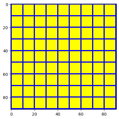
Make a grid of one blue line, every 10 rows and columns and display it

img = np.zeros((91,91,3), dtype=np.uint8 )
#plt.figure()
#plt.imshow( img )

img_white = img + 255
#plt.figure()
#plt.imshow( img_white )

## yellow (255, 255, 0)
img_yellow = img.copy() 
img_yellow[:,:,0:2] = 255
#plt.figure()
#plt.imshow( img_yellow )

print(f"First pixel values: {img_yellow[0,0,:]}")
print(f"Last pixel values: {img_yellow[-1,-1,:]}")

img_yellow[::10,:,:] = (0, 0, 255)
img_yellow[:,::10,:] = (0, 0, 255)
plt.figure()
plt.imshow(img_yellow)

First pixel values: [255 255   0]
Last pixel values: [255 255   0]

<matplotlib.image.AxesImage at 0x7ccd006468f0>

Exercise 2#

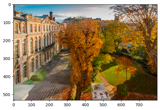
With the function plt.imread read the file les-mines.jpg or any other image
or any other image - just pay attention to the size.
Check if the object is editable with im.flags.writeable.
if it is not, copy it
Display the image
What is the type of the object created?
What is the size of the image?
What is the size of the image in height and width?
What is the number of bytes used per pixel?
What is the type of the pixels?
(two types for the pixels: 8-bit unsigned integers or 64-bit floats)
What are its maximum and minimum pixel values?
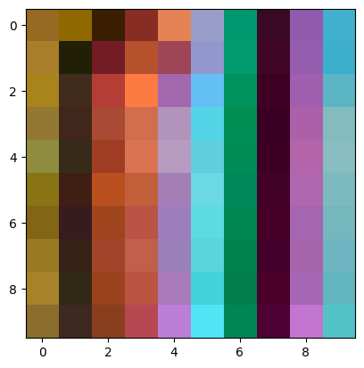
Show the 10 x 10 pixel rectangle at the top of the image

img = plt.imread( "media/les-mines.jpg")
plt.imshow( img )
print(f"editable: {img.flags.writeable}")
if not img.flags.writeable:
    img2 = np.copy(img)
else:
    img2 = img 
    
print(f"Image {img2.shape[0]}x{img2.shape[1]} (height x width)")
print(f"Number of bytes for one pixel: {img2.itemsize}")
print(f"Pixel type: {img2.dtype}")
print(f"Min pixel: {img2.min()} - Max pixel: {img2.max()}")
plt.figure()
plt.imshow( img2[:10, :10,:])

editable: False
Image 533x800 (height x width)
Number of bytes for one pixel: 1
Pixel type: uint8
Min pixel: 0 - Max pixel: 255

<matplotlib.image.AxesImage at 0x7ccd0058a8c0>

Exercise 3#

reminder RGB-A

you can indicate, in a fourth value of the pixels, their transparency
this 4th channel is called the alpha channel
the values go from 0 for transparent to 255 for opaque

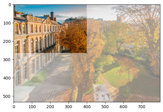
Rereading the initial image (without copying it)
Create an empty array of the same height and width as the image, of the same type as the original image, with a fourth channel
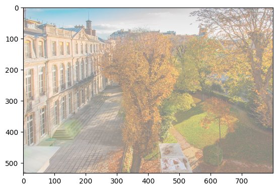
Copy the original image into it, set the fourth channel to 128 and display the image

img = plt.imread("media/les-mines.jpg")
alpha_img = np.empty( (img.shape[0], img.shape[1], 4), dtype=np.uint8)
alpha_img[:,:,:3] = img
alpha_img[:,:,3] = 128 
plt.imshow( alpha_img )
plt.figure()
nx,ny = alpha_img.shape[:2]
alpha_img[:(nx//2),:(ny//2),3] = 255
plt.imshow(alpha_img)

<matplotlib.image.AxesImage at 0x7ccd00179450>

Exercise 4 - gray scale#

Read the image les-mines.jpg
Pass its values in floats between 0 and 1 and display it
Transform the image into two grayscale images :
a. by averaging the R, G, B values for each pixel
b. using the ‘Y’ correction (which corrects the constrate) based on the formula
G = 0.299 * R + 0.587 * V + 0.114 * B
Square the pixels and display the image
Root the pixels and display it
Convert the grayscale image to 8-bit unsigned integer type and display it
in grayscale

Exercice 5 - sepia#

To change the R, G and B values of a pixel to sepia
(encoded here on an 8 bits unsigned integer)

we transform the values $R$, $G$ and $B$ by the transformation
$0.393\, R + 0.769\, G + 0.189\, B$
$0.349\, R + 0.686\, G + 0.168\, B$
$0.272\, R + 0.534\, G + 0.131\, B$
(attention the calculations must be done in floats not in uint8
to avoid having, for example, 256 becoming 0)
then we threshold the values which are greater than 255 to 255.
of course the image must then be put back in a correct format
(uint8 or float between 0 and 1)

Exercise 6 - Compress the image with SVD#

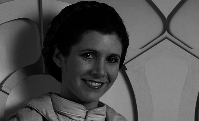
In this exercise the objective is to compress a grayscale image using an SVD (Singular Value Decomposition). The image to be compressed is the following :

As a reminder, the SVD decomposition of a matrix $\mathbf{A} \in \mathbb{R}^{m \times n}$ is written as follows:

\[ \mathbf{A} = \mathbf{U}\cdot\mathbf{\Sigma}\cdot\mathbf{V} \]

With $\mathbf{U}\in \mathbb{R}^{m\times m}$, $\mathbf{\Sigma}\in \mathbb{R}^{m\times n}$ a diagonal matrix of singular values and $\mathbf{V} \in \mathbb{R}^{n\times n}$.

Question 1:

Load the image of Carrie Fisher (you will find in the data folder a file carrie_fisher.npy containing the image in the form of an np.ndarray) and calculate its decomposition into singular values.

Question 2 :

Draw the evolution of the singular values of the image.

Question 3 :

For different truncations ($k=\lbrace 1,5,10,15,20,30,50,100 \rbrace$) reconstruct the image, display it and compute the compression ratio obtained.

Scipy exercises#

EDO solution#

Consider a classical RC circuit defined by the following differential equation:

\[ RC \frac{du}{dt} + u = u_e \]

\[ \frac{du}{dt} = \frac{u_e - u }{RC} \]

With $R=1000\Omega$, $C=10^{-6}F$ and $u(t=0) = 0$.

Question 1:

In the case where $u_e(t) = U_0$ with $U_0=10\,V$ calculate the solution of the differential equation on the interval $[0, 0.005]$.

Question 2:

In the case $u_e(t) = U_0 \sin \left( 2\pi f t \right)$ with $U_0=10\,V$ and $f=100\,Hz$ calculate the solution of the differential equation on the interval $[0, 5/f]$.

Solve a system of differential equation#

Consider a classical RLC circuit defined by the following differential equation:

\[LC\frac{d^2u}{dt^2} + RC \frac{du}{dt} + u = u_e \]

Question 1:

Transform this second order equation into a system of two first order equations.

Question 2 :

Determine the evolution of $u(t)$ on the interval $t \in [0, 0.02]$ for $R=1000\,\Omega$, $F=10^{-6}\,F$. It is up to you to choose the value of $L$ to solve: (i) pseudo-periodic; (ii) aperiodic; (iii) critical.

As a reminder: $$q = \frac{1}{R} \sqrt{ \frac{L}{C} } \; ; \begin{cases} q = \dfrac{1}{2} & critical \\ q < \dfrac{1}{2} & aperiodiue \\ q > \dfrac{1}{2} & pseudo-periodic \\ \end{cases} $$

If you want to use ipywidgets (you have to install it via conda) you can make an interactive graph with the value of $L$.

Find the zero of a scalar function#

Consider the Kepler equation:

\[ x - e\cdot \sin x = m \]

Question 1:

Using scipy find the solution of the Kepler equation in the case where $e=\frac{1}{2}$ and $m=1$. Check that the solution found by scipy is correct.

Parameter assignment — RC circuit#

Let’s consider the RC circuit previously studied.

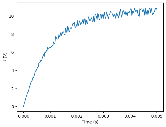
We will try to identify the parameter R of the system from “experimental” data. The experimental data in question are given in the file notebook/data/exp_data_rc.dat. If we represent these data we obtain the following curve:

import matplotlib.pyplot as plt 
import numpy as np
import pathlib as pl 

data = np.loadtxt(str(pl.Path(".") / "data" / "exp_data_rc.dat"))

plt.plot( data[:,0], data[:,1])
plt.xlabel("Time (s)")
plt.ylabel("U (V)")
plt.show()

This data is obtained with the following configuration:

\[ u_e = 10\,V\, ; \, C=10^{-6}\,F\, ; \, R=?? \]

Question 1: Formulate the optimization problem to be solved to identify the parameter R ?

Question 2: Using scipy.optimize identify the value of the R parameter.

Question 3: Plot on the same graph the experimental data and the model result for the identified value of $R$.

Python for Engineers

Course exercises

Contents

Course exercises#

Exercise on slicing#

Exercises on strings#

Exercise 1#

Exercises 2#

Exercise on lists#

Exercise on dictionaries#

Exercises on functions#

Exercise 1#

Exercise 2#

Exercises on classes#

Exercise 1#

Exercise 2#

Numpy exercise#

Data manipulation#

Images#

Exercise 1#

Exercise 2#

Exercise 3#

Exercise 4 - gray scale#

Exercice 5 - sepia#

Exercise 6 - Compress the image with SVD#

Scipy exercises#

EDO solution#

Solve a system of differential equation#

Find the zero of a scalar function#

Parameter assignment — RC circuit#